Answer
Empirically the first_sum implementation is the slowest and the third_sum implementation is the
fastest.
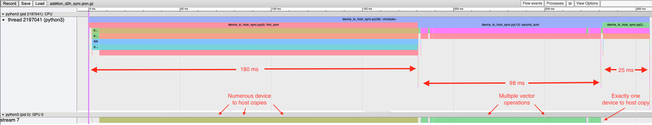
PyTorch profiler trace for first_sum, second_sum and third_sum
The trace above shows that duration of each function and highlights the numerous device-to-host
memory copy kernels triggered in the first_sum implementation and the various vector ops taking
place in the second_sum function and the single device-to-host copy in third_sum. The trace file is available
here.
Analyzing first_sum - numerous device to host copies
def first_sum(cuda_tensor):
    total = 0.0
    for i in range(cuda_tensor.size()[0]):
        total += cuda_tensor[i].cpu()
    return total
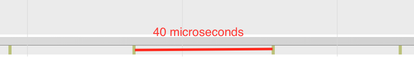
Zoomed view - first_sum
In the first_sum function the number of copies from the device to the host is equal to the size of
the tensor. These are incurred due to the .cpu() call in the for loop. Each .cpu() call moves a
small amount of data from the GPU to the CPU and takes about $1$ microsecond. Additionally, the gap betweeen
consecutive kernels is about $40$ microseconds. These repeated calls,
highighted in the zoomed trace above make the first_sum implementation the slowest one.
Analyzing second_sum - no device to host copies
def second_sum(cuda_tensor):
    total = torch.zeros(1, device='cuda')
    for i in range(cuda_tensor.size()[0]):
        total += cuda_tensor[i]
    return total

Zoomed view - second_sum
The second_sum function initializes and places the total tensor on the GPU. Addition of each
element of a_tensor to total triggers vector op kernels. The addition is slowed due to the launch
overhead of these kernels. The arithmetic intensity of vector ops involving small tensors is low and
such operations can be done on the CPU, when reasonable. Even though there are no instances of
device to host copies and synchronizations in the second_sum implementation, the GPU is
considerably underutilized. This can be seen by the $\sim 20$ microsecond gaps between consecutive kernels
on stream $7$.
Analyzing third_sum - addition on the CPU
def third_sum(cuda_tensor):
    total = 0.0
    tensor_on_cpu = cuda_tensor.cpu()
    for i in range(tensor_on_cpu.size()[0]):
        total += tensor_on_cpu[i]
    return total
Finally, the third_sum implementation copies the entire tensor to the CPU and pays a small one
time cost to transfer data. Precisely speaking, $4 \times 4096$ bytes are transferred in $2$ microseconds.
Thus the achieved PCIe bandwidth is approximately $8$ GB/sec. The summation is done on the CPU as
total and the elements of the tensor are on the CPU. It is extremely slow due to lack of
instruction-level and core-level parallelism and the additional PyTorch overhead makes it even
slower.
Discussion
What is the fastest way to add in PyTorch?
torch.sum has better performance than the above implementations. The functions above are contrived
examples to demonstrate device-to-host synchronization and launch overhead. The table below
summarizes the time taken by the three functions above and torch.sum.
| function | CPU time (ms) | GPU time(ms) |
|---|---|---|
| first_sum | 183 | 181 |
| second_sum | 87 | 86 |
| third_sum | 25 | 0.001 |
| torch.sum() (tensor on GPU) | 0.161 | 0.009 |
| torch.sum() (tensor on CPU) | 1.8 | NA |
torch.sum() uses Intel Math Kernel Library (MKL) to sum the tensors which fully utilizes the cores
and instruction-level parallelism to speed up the computation. Intel MKL is written in C++ so there
is no Python overhead either.
What is synchronization?
There are three levels of synchronization: Device synchronization, Stream synchronization and Event synchronization.
A stream is a sequence of operations that are performed in order on the device. Operations in different streams can be interleaved and in some cases overlapped - a property that can be used to hide data transfers between the host and the device. For more details on streams check out Swimming in Streams.
A CUDA event is a synchronization marker that can be used to monitor the device’s progress, to accurately measure timing, and to synchronize CUDA streams.
-
Using
torch.cuda.synchronize()leads to device synchronization which blocks execution on the CPU thread until the device has completed all preceding tasks. It waits for the GPU to finish kernel execution on all streams. -
CUDA streams can be synchronized using
torch.cuda.Stream.synchronize(). Execution is blocked on the CPU thread until the device has executed all kernels on the specified stream. -
Event synchronization can be triggered using
torch.cuda.Event.synchronize(). It prevents the CPU thread from proceeding until the event is completed.
What are some naturally occurring synchronization points in PyTorch?
- Explicit call to
torch.cuda.synchronize(). - Implicity the following calls trigger synchronization:
.item(),.cpu(),torch.nonzero,torch.masked_select. - Logging statements from the GPU.
Why are there thousands of calls to cudaStreamSynchronize in the trace?
-
Iterating over a for loop as in
first_sumcauses synchronization and leads to performance degradation. These synchronization points are visible and avoidable. A better implementation would parallelize the computation by launching multiple threads rather than iterating over it. -
As seen in the
second_sum, an absence of synchronization points does not guarantee good performance. Executing multiple small kernels iteratively does not utilize the GPU completely. -
Synchronization points can stall the CUDA launch queue which can make the job CPU bound. More about this in the next post.
How can I find synchronization points in my program?
Use
torch.cuda.set_sync_debug_mode(),
when possible. Currently, this feature does not support torch.distributed and torch.sparse
namespaces.
Analyzing traces with Holistic Trace Analysis
Looking at the trace, you may note that the cudaMemcpyAsync event on the CPU has a longer duration
than the corresponding operation (MemcpyDtoH) on the GPU. This may not be easy to find in general.
The Holistic Trace Analysis (HTA)
library provides a convenient way to identify this behavior using the Cuda Kernel Launch
Statistics
feature. Using the PyTorch profiler traces, HTA provides insights for performance debugging. The
get_cuda_kernel_launch_stats
function displays the distribution of GPU kernels (in particular, cudaLaunchKernel,
cudaMemcpyAsync and cudaMemsetAsync) whose duration is less than the corresponding CPU event.
Profiling each function as an independent python program we generated three traces and analyzed them
with the get_cuda_kernel_launch_stats feature. One of the outputs from the
get_cuda_kernel_launch_stats function are the graphs below which show that there are thousands of
GPU events with duration shorter than the corresponding CPU event, thus highlighting the issues with
the first_sum and second_sum implementations.
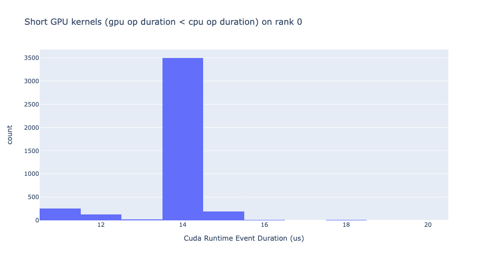
Cuda Kernel Launch Stats - first_sum
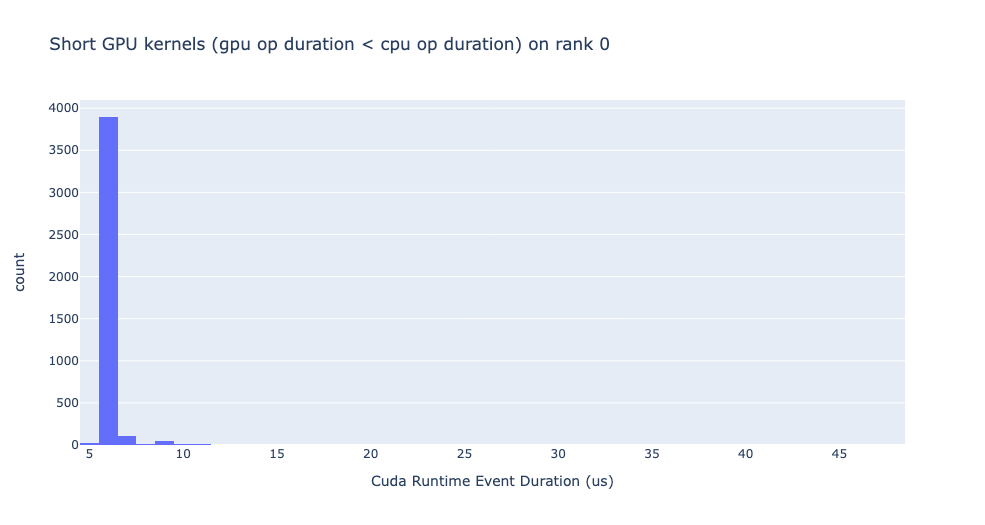
Cuda Kernel Launch Stats - second_sum
The graphs above were generated using the following code snippet:
from hta.trace_analysis import traceanalysis
analyzer = traceanalysis(trace_dir = "/path/to/trace/folder")
kernel_stats = analyzer.get_cuda_kernel_launch_stats()
Here are the traces for the first_sum, second_sum and third_sum functions.
What should you remember in years to come?
- Multiple small repeated kernel calls or device-to-host copies make your code perform poorly. They can often be replaced this with a single large compute/copy kernel.
- Be aware of device-to-host synchronization points since they can often be avoided.
Explore more
- Find the kernels taking the most time in your model using the Kernel Breakdown feature in Holistic Trace Analysis.
- Build a roofline model to find if the kernels are compute bound or memory bandwidth bound.